4 Examples
Following are some examples to demonstrate as well as test the correctness of the error
propagation algorithm of Section 3. In the following examples, various functions are written
in different algebraic forms and the results for the different forms is shown to be exactly same
(e.g. cos(x) vs. 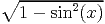 , tan(x) vs. sin(x)∕ cos(x)). These examples also verify that
the combination of a function and its inverse simply returns the argument (e.g
asin(sin(x)) = x), as well as functions like sinh(x)∕((exp(x) - exp(-x))∕2) (which is really a
complicated way of writing 1!) returns a value of 1 with no error. However, if the values
of two independent variates x1 and x2 and their corresponding errors are same,
the value of expressions like sin 2(x
1) + cos 2(x
2) will be 1 but the error will not be
zero.
, tan(x) vs. sin(x)∕ cos(x)). These examples also verify that
the combination of a function and its inverse simply returns the argument (e.g
asin(sin(x)) = x), as well as functions like sinh(x)∕((exp(x) - exp(-x))∕2) (which is really a
complicated way of writing 1!) returns a value of 1 with no error. However, if the values
of two independent variates x1 and x2 and their corresponding errors are same,
the value of expressions like sin 2(x
1) + cos 2(x
2) will be 1 but the error will not be
zero.
Value of x = 1.00000 +/- 0.10000
Value of y = 2.00000 +/- 0.20000
Value of x1 = 1.00000 +/- 0.10000
Value of x2 = 1.00000 +/- 0.10000
sin(x) = 0.84147 +/- 0.05403
sqrt(1-sin(x)^2) = 0.54030 +/- 0.08415
cos(x) = 0.54030 +/- 0.08415
tan(x) = 1.55741 +/- 0.34255
sin(x)/cos(x) = 1.55741 +/- 0.34255
asin(sin(x)) = 1.00000 +/- 0.10000
asinh(sinh(x)) = 1.00000 +/- 0.10000
atanh(tanh(x)) = 1.00000 +/- 0.10000
exp(ln(x)) = 1.00000 +/- 0.10000
sinh(x) = 1.17520 +/- 0.15431
(exp(x)-exp(-x))/2 = 1.17520 +/- 0.15431
sinh(x)/((exp(x)-exp(-x))/2) = 1.00000
x/exp(ln(x)) = 1.00000
sin(x1)⋆sin(x1) = 0.70807 +/- 0.09093
sin(x1)⋆sin(x2) = 0.70807 +/- 0.06430
sin(x1)^2+cos(x1)^2 = 1.00000 +/- 0.00000
sin(x1)^2+cos(x2)^2 = 1.00000 +/- 0.12859
4.1 Recursion
Following is an example of error propagation in a recursive function. The factorial of x is written
as a recursive function f(x). Its derivative is given by f(x)![[1 + -1- + -1-+ ⋅⋅⋅ + 1 + 1]
x x- 1 x- 2 2](fussy15x.png) . The
term in the parenthesis is also written as a recursive function df(x). It is shown that the
propagated error in f(x) is equal to f(x)df(x)δx.
. The
term in the parenthesis is also written as a recursive function df(x). It is shown that the
propagated error in f(x) is equal to f(x)df(x)δx.
>f(x) {if (x==1) return x; else return x⋆f(--x);}
>df(x){if (x==1) return x; else return 1/x+df(--x);}
>f(x=10pm1)
3628800.00000 +/- 10628640.00000
>(f(x)⋆df(x)⋆x.rms).val
10628640.00000
Similarly, the recurrence relations for the Laguerre polynomial of order n and its derivative
evaluated at x are given by
These are written as recursive functions l(n,x) and dl(n,x) and it is shown that the
propagated error in Ln(x) is equal to Ln′(x)δx.
>l(n,x){
if (n<=0) return 1;
if (n==1) return 1-x;
return ((2⋆n-1-x)⋆l(n-1,x)-(n-1)⋆l(n-2,x))/n;
}
>dl(n,x){return (n/x)⋆(l(n,x)-l(n-1,x));}
>l(4,x=3pm1)
1.37500 +/- 0.50000
>(dl(4,x)⋆x.rms).val
0.50000
![(
{ 1 n = 0
L (x ) = 1 - x n = 1 (5)
n ( (2n--1-x)Ln-1(x)--(n--1)Ln-2(x)
n n ≥ 2
L′n (x ) = (n∕x) [Ln (x) - Ln-1(x )] (6)](fussy16x.png)